2 Knoten- Spannungs- Analyse

Die Knoten-Spannungsanalyse ist eine Methode zur Berechnung der unbekannten elektrischen Größen in einem Netzwerk von elektrischen oder elektronischen Komponenten.
Unter Verwendung der Knotenregel, der Maschenregel und dem Ohmschen Gesetz werden Gleichungen aufgestellt, welche die Schaltung rechnerisch beschreiben. Es entsteht ein lineares Gleichungssystem, das gelöst werden kann.

2.1 Beispiel 1

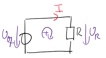
In Grafik Abbildung 2.1 ist ein Netzwerk aus Widerständen und Spannungsquellen dargestellt.

Vorgehensweise
1. Alle Ströme und Spannungen einzeichnen
2. Unbekannte Größen definieren

\(R\) … Widerstand

\(U_{q}\) … Quellspannung

\(U_{R}\) … Spannungsabfall am Widerstand

\(I\) … Strom

3. Knoten und Maschen einzeichnen
Siehe Abbildung 2.1
4. Knoten- und Maschengleichungen aufstellen

Maschengleichungen

\(\displaystyle 0 = U_{R} - U_{q}\)

Knotengleichungen

Es gibt keinen Knoten

5. Ohmsche Gesetze für die Widerstände anschreiben

Ohmsches Gesetz

\(\displaystyle U_{R} = I R\)

6. Überprüfen, ob es gleich viele Gleichungen wie Unbekannte gibt
Passt, es gibt 2 Gleichungen und 2 Unbekannte.

7. Gleichungssystem lösen
Das Gleichungssystem kann mit der Hand gelöst werden. Für komplexere Schaltungen ist es sinnvoll, ein Computerprogramm zu verwenden.

\(\displaystyle U_{R} = U_{q}\)

\(\displaystyle I = \frac{U_{q}}{R}\)

Für so eine einfache Schaltung würde man die Knoten-Spannungs-Analyse nicht verwenden. Die Methode lässt sich allerdings auf beliebig Komplexe Schaltungen anwenden.

2.2 Beispiel 2

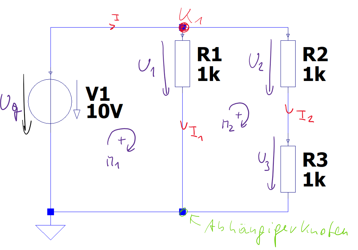
In Grafik Abbildung 2.2 ist ein Netzwerk aus Widerständen und Spannungsquellen dargestellt.

Vorgehensweise
1. Alle Ströme und Spannungen einzeichnen
2. Unbekannte Größen definieren

\(R_{1}\) … Widerstand 1

\(R_{2}\) … Widerstand 2

\(R_{3}\) … Widerstand 3

\(U_{q}\) … Quellspannung

\(U_{1}\) … Spannungsabfall an R1

\(U_{2}\) … Spannungsabfall an R2

\(U_{3}\) … Spannungsabfall an R3

\(I_{1}\) … Strom durch R1

\(I_{2}\) … Strom durch R2

\(I\) … Gesamtstrom

3. Knoten und Maschen einzeichnen
Siehe Abbildung 2.2
4. Knoten- und Maschengleichungen aufstellen

Maschengleichungen

\[ 0 = U_{1} - U_{q} \tag{2.1}\]

\[ 0 = - U_{1} + U_{2} + U_{3} \tag{2.2}\]

Knotengleichungen

\[ 0 = I - I_{1} - I_{2} \tag{2.3}\]

5. Ohmsche Gesetze für die Widerstände anschreiben

Ohmsches Gesetz

\[ U_{1} = I_{1} R_{1} \tag{2.4}\]

\[ U_{2} = I_{2} R_{2} \tag{2.5}\]

\[ U_{3} = I_{2} R_{3} \tag{2.6}\]

6. Überprüfen ob es gleich viele Gleichungen wie Unbekannte gibt
Passt, es gibt 6 Gleichungen und 6 Unbekannte.

7. Gleichungssystem lösen
Das Gleichungssystem kann mit der Hand gelöst werden. Für komplexere Schaltungen ist es sinnvoll, ein Computerprogramm zu verwenden.

\[ U_{1} = U_{q} \tag{2.7}\]

\[U_{1} = \mathtt{\text{10}} \ \mathtt{\text{V}}\]

\[ U_{2} = \frac{R_{2} U_{q}}{R_{2} + R_{3}} \tag{2.8}\]

\[U_{2} = \mathtt{\text{5}} \ \mathtt{\text{V}}\]

\[ U_{3} = \frac{R_{3} U_{q}}{R_{2} + R_{3}} \tag{2.9}\]

\[U_{3} = \mathtt{\text{5}} \ \mathtt{\text{V}}\]

\[ I_{1} = \frac{U_{q}}{R_{1}} \tag{2.10}\]

\[I_{1} = \mathtt{\text{10}} \ \mathtt{\text{mA}}\]

\[ I_{2} = \frac{U_{q}}{R_{2} + R_{3}} \tag{2.11}\]

\[I_{2} = \mathtt{\text{5}} \ \mathtt{\text{mA}}\]

\[ I = \frac{R_{1} U_{q} + R_{2} U_{q} + R_{3} U_{q}}{R_{1} R_{2} + R_{1} R_{3}} \tag{2.12}\]

\[I = \mathtt{\text{15}} \ \mathtt{\text{mA}}\]

2.3 Beispiel 3

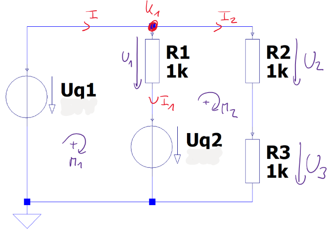
In Grafik Abbildung 2.3 ist ein Netzwerk aus Widerständen und Spannungsquellen dargestellt.

2.3.1 Alle Ströme und Spannungen einzeichnen

2.3.2 Bekannte Größen

\[R_{1} = \mathtt{\text{1}} \ \mathrm{k\Omega}\]

\[R_{2} = \mathtt{\text{1}} \ \mathrm{k\Omega}\]

\[R_{3} = \mathtt{\text{1}} \ \mathrm{k\Omega}\]

\[U_{q1} = \mathtt{\text{10}} \ \mathtt{\text{V}}\]

\[U_{q2} = \mathtt{\text{1}} \ \mathtt{\text{V}}\]

2.3.3 Unbekannte Größen definieren

\(U_{1}\) … Spannungsabfall an R1

\(U_{2}\) … Spannungsabfall an R2

\(U_{3}\) … Spannungsabfall an R3

\(I_{1}\) … Strom durch R1

\(I_{2}\) … Strom durch R2

\(I\) … Gesamtstrom

2.3.4 Knoten und Maschen einzeichnen

Siehe Abbildung 2.3

2.3.5 Knoten- und Maschengleichungen aufstellen

Maschengleichungen

\[ 0 = U_{1} - U_{q1} + U_{q2} \tag{2.13}\]

\[ 0 = - U_{1} + U_{2} + U_{3} - U_{q2} \tag{2.14}\]

Knotengleichungen

\[ 0 = I - I_{1} - I_{2} \tag{2.15}\]

2.3.6 Ohmsche Gesetze für die Widerstände anschreiben

Ohmsches Gesetz

\[ U_{1} = I_{1} R_{1} \tag{2.16}\]

\[ U_{2} = I_{2} R_{2} \tag{2.17}\]

\[ U_{3} = I_{2} R_{3} \tag{2.18}\]

2.3.7 Überprüfen ob es gleich viele Gleichungen wie Unbekannte gibt

Passt, es gibt 6 Gleichungen und 6 Unbekannte.

2.3.8 Gleichungssystem lösen

Das Gleichungssystem kann mit der Hand gelöst werden. Für komplexere Schaltungen ist es sinnvoll, ein Computerprogramm zu verwenden.

\[ U_{1} = U_{q1} - U_{q2} \tag{2.19}\]

\[U_{1} = \mathtt{\text{9}} \ \mathtt{\text{V}}\]

\[ U_{2} = \frac{R_{2} U_{q1}}{R_{2} + R_{3}} \tag{2.20}\]

\[U_{2} = \mathtt{\text{5}} \ \mathtt{\text{V}}\]

\[ U_{3} = \frac{R_{3} U_{q1}}{R_{2} + R_{3}} \tag{2.21}\]

\[U_{3} = \mathtt{\text{5}} \ \mathtt{\text{V}}\]

\[ I_{1} = \frac{U_{q1} - U_{q2}}{R_{1}} \tag{2.22}\]

\[I_{1} = \mathtt{\text{9}} \ \mathtt{\text{mA}}\]

\[ I_{2} = \frac{U_{q1}}{R_{2} + R_{3}} \tag{2.23}\]

\[I_{2} = \mathtt{\text{5}} \ \mathtt{\text{mA}}\]

\[ I = \frac{R_{1} U_{q1} + R_{2} U_{q1} - R_{2} U_{q2} + R_{3} U_{q1} - R_{3} U_{q2}}{R_{1} R_{2} + R_{1} R_{3}} \tag{2.24}\]

\[I = \mathtt{\text{14}} \ \mathtt{\text{mA}}\]

2.4 Beispiel 4

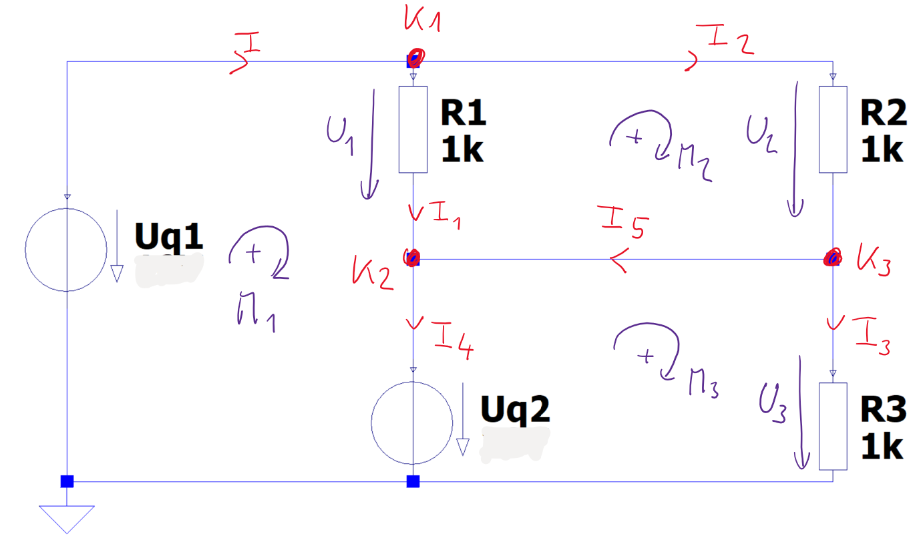
In Grafik Abbildung 2.4 ist ein Netzwerk aus Widerständen und Spannungsquellen dargestellt.

Vorgehensweise
1. Alle Ströme und Spannungen einzeichnen
2. Unbekannte Größen definieren

Bekannte Größen

\(R_{1}\) … Widerstand 1

\(R_{2}\) … Widerstand 2

\(R_{3}\) … Widerstand 3

\(U_{q1}\) … Quellspannung

\(U_{q2}\) … Quellspannung

\[R_{1} = \mathtt{\text{1}} \ \mathrm{k\Omega}\]

\[R_{2} = \mathtt{\text{1}} \ \mathrm{k\Omega}\]

\[R_{3} = \mathtt{\text{1}} \ \mathrm{k\Omega}\]

\[U_{q1} = \mathtt{\text{10}} \ \mathtt{\text{V}}\]

\[U_{q2} = \mathtt{\text{1}} \ \mathtt{\text{V}}\]

Unbekannte Größen

\(U_{1}\) … Spannungsabfall an R1

\(U_{2}\) … Spannungsabfall an R2

\(U_{3}\) … Spannungsabfall an R3

\(I_{1}\) … Strom durch R1

\(I_{2}\) … Strom durch R2

\(I_{3}\) … Strom durch R3

\(I_{4}\) … Strom durch Quelle \(U_{q2}\)

\(I_{5}\) … Querstrom

\(I\) … Gesamtstrom

3. Knoten und Maschen einzeichnen
Siehe Abbildung 2.4

4. Knoten- und Maschengleichungen aufstellen

Maschengleichungen

\[ 0 = U_{1} - U_{q1} + U_{q2} \tag{2.25}\]

\[ 0 = - U_{1} + U_{2} \tag{2.26}\]

\[ 0 = U_{3} - U_{q2} \tag{2.27}\]

Knotengleichungen

\[ 0 = I - I_{1} - I_{2} \tag{2.28}\]

\[ 0 = I_{1} - I_{4} + I_{5} \tag{2.29}\]

\[ 0 = I_{2} - I_{3} - I_{5} \tag{2.30}\]

5. Ohmsche Gesetze für die Widerstände anschreiben

Ohmsches Gesetz

\[ U_{1} = I_{1} R_{1} \tag{2.31}\]

\[ U_{2} = I_{2} R_{2} \tag{2.32}\]

\[ U_{3} = I_{3} R_{3} \tag{2.33}\]

6. Überprüfen ob es gleich viele Gleichungen wie Unbekannte gibt
Passt, es gibt 9 Gleichungen und 9 Unbekannte.

7. Gleichungssystem lösen
Das Gleichungssystem kann mit der Hand gelöst werden. Für komplexere Schaltungen ist es sinnvoll, ein Computerprogramm zu verwenden.

\[ U_{1} = U_{q1} - U_{q2} \tag{2.34}\]

\[U_{1} = \mathtt{\text{9}} \ \mathtt{\text{V}}\]

\[ U_{2} = U_{q1} - U_{q2} \tag{2.35}\]

\[U_{2} = \mathtt{\text{9}} \ \mathtt{\text{V}}\]

\[ U_{3} = U_{q2} \tag{2.36}\]

\[U_{3} = \mathtt{\text{1}} \ \mathtt{\text{V}}\]

\[ I_{1} = \frac{U_{q1} - U_{q2}}{R_{1}} \tag{2.37}\]

\[I_{1} = \mathtt{\text{9}} \ \mathtt{\text{mA}}\]

\[ I_{2} = \frac{U_{q1} - U_{q2}}{R_{2}} \tag{2.38}\]

\[I_{2} = \mathtt{\text{9}} \ \mathtt{\text{mA}}\]

\[ I_{3} = \frac{U_{q2}}{R_{3}} \tag{2.39}\]

\[I_{3} = \mathtt{\text{1}} \ \mathtt{\text{mA}}\]

\[ I_{4} = \frac{- R_{1} R_{2} U_{q2} + R_{1} R_{3} U_{q1} - R_{1} R_{3} U_{q2} + R_{2} R_{3} U_{q1} - R_{2} R_{3} U_{q2}}{R_{1} R_{2} R_{3}} \tag{2.40}\]

\[I_{4} = \mathtt{\text{17}} \ \mathtt{\text{mA}}\]

\[ I_{5} = \frac{- R_{2} U_{q2} + R_{3} U_{q1} - R_{3} U_{q2}}{R_{2} R_{3}} \tag{2.41}\]

\[I_{5} = \mathtt{\text{8}} \ \mathtt{\text{mA}}\]

\[ I = \frac{R_{1} U_{q1} - R_{1} U_{q2} + R_{2} U_{q1} - R_{2} U_{q2}}{R_{1} R_{2}} \tag{2.42}\]

\[I = \mathtt{\text{18}} \ \mathtt{\text{mA}}\]

2.5 Beispiel 5

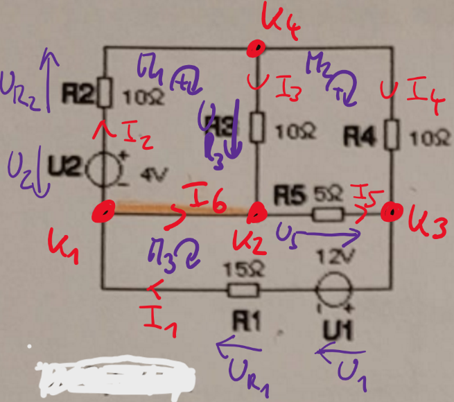
In Grafik Abbildung 2.5 ist ein Netzwerk aus Widerständen und Spannungsquellen dargestellt.

Vorgehensweise
1. Alle Ströme und Spannungen einzeichnen
2. Unbekannte Größen definieren

Code

from sympy import *

# Variablen
R1 = MySymbol('R1',description='Widerstand 1',unit=u.ohm,value=15)
R2 = MySymbol('R2',description='Widerstand 2',unit=u.ohm,value=10)
R3 = MySymbol('R3',description='Widerstand 3',unit=u.ohm,value=10)
R4 = MySymbol('R4',description='Widerstand 3',unit=u.ohm,value=10)
R5 = MySymbol('R5',description='Widerstand 3',unit=u.ohm,value=5)
U1 = MySymbol('U_1',description='Quellspannung',unit=u.V,value=12)
U2 = MySymbol('U_2',description='Quellspannung',unit=u.V,value=4)
UR1 = MySymbol('U_R1',description='Spannungsabfall an R1',unit=u.V)
UR2 = MySymbol('U_R2',description='Spannungsabfall an R2',unit=u.V)
UR3 = MySymbol('U_R3',description='Spannungsabfall an R3',unit=u.V)
UR4 = MySymbol('U_R4',description='Spannungsabfall an R4',unit=u.V)
UR5 = MySymbol('U_R5',description='Spannungsabfall an R5',unit=u.V)
I1 = MySymbol('I1',description='Strom durch R1',unit=u.A)
I2 = MySymbol('I2',description='Strom durch R2',unit=u.A)
I3 = MySymbol('I3',description='Strom durch R3',unit=u.A)
I4 = MySymbol('I4',description='Strom durch R4',unit=u.A)
I5 = MySymbol('I5',description='Strom durch R5',unit=u.A)
I6 = MySymbol('I6',description='Querstrom',unit=u.A)

display(Markdown('**Bekannte Größen**'))
knowns = [R1,R2,R3,R4,R5,U1,U2]
QBookHelpers.print_description(knowns)
QBookHelpers.print_values(knowns)
display(Markdown('Anzahl der bekannten Größen:'))
display(len(knowns))

display(Markdown('**Unbekannte Größen**'))
unknowns = [UR1,UR2,UR3,UR4,UR5,I1,I2,I3,I4,I5,I6]
QBookHelpers.print_description(unknowns)
display(Markdown('Anzahl der unbekannten Größen:'))
display(len(unknowns))

Bekannte Größen

\(R_{1}\) … Widerstand 1

\(R_{2}\) … Widerstand 2

\(R_{3}\) … Widerstand 3

\(R_{4}\) … Widerstand 3

\(R_{5}\) … Widerstand 3

\(U_{1}\) … Quellspannung

\(U_{2}\) … Quellspannung

\[R_{1} = \mathtt{\text{15}} \ \mathrm{\Omega}\]

\[R_{2} = \mathtt{\text{10}} \ \mathrm{\Omega}\]

\[R_{3} = \mathtt{\text{10}} \ \mathrm{\Omega}\]

\[R_{4} = \mathtt{\text{10}} \ \mathrm{\Omega}\]

\[R_{5} = \mathtt{\text{5}} \ \mathrm{\Omega}\]

\[U_{1} = \mathtt{\text{12}} \ \mathtt{\text{V}}\]

\[U_{2} = \mathtt{\text{4}} \ \mathtt{\text{V}}\]

Anzahl der bekannten Größen:

Unbekannte Größen

\(U_{R1}\) … Spannungsabfall an R1

\(U_{R2}\) … Spannungsabfall an R2

\(U_{R3}\) … Spannungsabfall an R3

\(U_{R4}\) … Spannungsabfall an R4

\(U_{R5}\) … Spannungsabfall an R5

\(I_{1}\) … Strom durch R1

\(I_{2}\) … Strom durch R2

\(I_{3}\) … Strom durch R3

\(I_{4}\) … Strom durch R4

\(I_{5}\) … Strom durch R5

\(I_{6}\) … Querstrom

Anzahl der unbekannten Größen:

3. Knoten und Maschen einzeichnen
Siehe Abbildung 2.5

4. Knoten- und Maschengleichungen aufstellen

Code

# Gleichungen
display(Markdown('Maschengleichungen'))
M1 = Eq(0, U1+UR1+UR5)
M2 = Eq(0, -UR5+UR4-UR3)
M3 = Eq(0, +UR3-U2+UR2)
QBookHelpers.print_equation(M1,label='eq-M1')
QBookHelpers.print_equation(M2,label='eq-M2')
QBookHelpers.print_equation(M3,label='eq-M3')

display(Markdown('Knotengleichungen'))
K1 = Eq(0, I1-I2-I6)
K2 = Eq(0, I6+I3-I5)
K3 = Eq(0, I4+I5-I1)
K4 = Eq(0, I2-I4-I3)

QBookHelpers.print_equation(K1,label='eq-K1')
QBookHelpers.print_equation(K2,label='eq-K2')
QBookHelpers.print_equation(K3,label='eq-K3')
QBookHelpers.print_equation(K4,label='eq-K4')

Maschengleichungen

\[ 0 = U_{1} + U_{R1} + U_{R5} \tag{2.43}\]

\[ 0 = - U_{R3} + U_{R4} - U_{R5} \tag{2.44}\]

\[ 0 = - U_{2} + U_{R2} + U_{R3} \tag{2.45}\]

Knotengleichungen

\[ 0 = I_{1} - I_{2} - I_{6} \tag{2.46}\]

\[ 0 = I_{3} - I_{5} + I_{6} \tag{2.47}\]

\[ 0 = - I_{1} + I_{4} + I_{5} \tag{2.48}\]

\[ 0 = I_{2} - I_{3} - I_{4} \tag{2.49}\]

5. Ohmsche Gesetze für die Widerstände anschreiben

Code

display(Markdown('Ohmsches Gesetz'))
O1 = Eq(UR1, R1*I1)
O2 = Eq(UR2, R2*I2)
O3 = Eq(UR3, R3*I3)
O4 = Eq(UR4, R4*I4)
O5 = Eq(UR5, R5*I5)
QBookHelpers.print_equation(O1,label='eq-O1')
QBookHelpers.print_equation(O2,label='eq-O2')
QBookHelpers.print_equation(O3, label='eq-O3')
QBookHelpers.print_equation(O4, label='eq-O4')
QBookHelpers.print_equation(O5, label='eq-O5')

equations = [M1,M2,M3,K1,K2,K3,K4,O1,O2,O3,O4,O5]
display(Markdown('Anzahl der Gleichungen:'))
display(len(equations))

Ohmsches Gesetz

\[ U_{R1} = I_{1} R_{1} \tag{2.50}\]

\[ U_{R2} = I_{2} R_{2} \tag{2.51}\]

\[ U_{R3} = I_{3} R_{3} \tag{2.52}\]

\[ U_{R4} = I_{4} R_{4} \tag{2.53}\]

\[ U_{R5} = I_{5} R_{5} \tag{2.54}\]

Anzahl der Gleichungen:

6. Überprüfen ob es gleich viele Gleichungen wie Unbekannte gibt

Code

display(Markdown('Anzahl der Gleichungen:'))
display(len(equations))
display(Markdown('Anzahl der Unbekannten:'))
display(len(unknowns))

if len(equations) > len(unknowns):
    display(Markdown('Das Gleichungssystem ist überbestimmt. Es gibt mehr Gleichungen als Unbekannte. Das bedeutet, dass Gleichungen abhängig sind. Eine Gleichung kann aus den anderen abgeleitet werden. Wird diese Gleichung aus dem Gleichungssystem entfernt, so ist das Gleichungssystem lösbar. Mit Sympy kann das Gleichungssystem gelöst werden. Die überflüssigen Gleichungen werden ignoriert.'))
elif len(equations) < len(unknowns):
    display(Markdown('Das Gleichungssystem ist unterbestimmt. Es gibt mehr Unbekannte als Gleichungen. Das Gleichungssystem kann nicht gelöst werden.'))
elif len(equations) == len(unknowns):
    display(Markdown('Das Gleichungssystem hat gleich viele Gleichungen wie Unbekannte. Es kann gelöst werden, sofern es nicht widersprüchlich ist'))
else:
    display(Markdown('Fehler'))

Anzahl der Gleichungen:

Anzahl der Unbekannten:

Das Gleichungssystem ist überbestimmt. Es gibt mehr Gleichungen als Unbekannte. Das bedeutet, dass Gleichungen abhängig sind. Eine Gleichung kann aus den anderen abgeleitet werden. Wird diese Gleichung aus dem Gleichungssystem entfernt, so ist das Gleichungssystem lösbar. Mit Sympy kann das Gleichungssystem gelöst werden. Die überflüssigen Gleichungen werden ignoriert.

7. Gleichungssystem lösen

Code

# Gleichungssystem lösen
sol = linsolve(equations,unknowns)
#display(sol)
if sol == EmptySet:
    display(Markdown('Das Gleichungssystem hat keine Lösung.'))
else:
    for unk in unknowns:
        eq = Eq(unk,sol.args[0][unknowns.index(unk)])
        QBookHelpers.print_equation(eq,label='eq-' + unk.name)
        QBookHelpers.calculate_num_value(eq)
        QBookHelpers.print_values([unk])

\[ U_{R1} = \frac{- R_{1} R_{2} R_{3} U_{1} - R_{1} R_{2} R_{4} U_{1} - R_{1} R_{2} R_{5} U_{1} - R_{1} R_{3} R_{4} U_{1} - R_{1} R_{3} R_{5} U_{1} + R_{1} R_{3} R_{5} U_{2}}{R_{1} R_{2} R_{3} + R_{1} R_{2} R_{4} + R_{1} R_{2} R_{5} + R_{1} R_{3} R_{4} + R_{1} R_{3} R_{5} + R_{2} R_{3} R_{5} + R_{2} R_{4} R_{5} + R_{3} R_{4} R_{5}} \tag{2.55}\]

\[U_{R1} = \mathtt{\text{-9.2}} \ \mathtt{\text{V}}\]

\[ U_{R2} = \frac{R_{1} R_{2} R_{3} U_{2} + R_{1} R_{2} R_{4} U_{2} + R_{1} R_{2} R_{5} U_{2} - R_{2} R_{3} R_{5} U_{1} + R_{2} R_{3} R_{5} U_{2} + R_{2} R_{4} R_{5} U_{2}}{R_{1} R_{2} R_{3} + R_{1} R_{2} R_{4} + R_{1} R_{2} R_{5} + R_{1} R_{3} R_{4} + R_{1} R_{3} R_{5} + R_{2} R_{3} R_{5} + R_{2} R_{4} R_{5} + R_{3} R_{4} R_{5}} \tag{2.56}\]

\[U_{R2} = \mathtt{\text{1.73}} \ \mathtt{\text{V}}\]

\[ U_{R3} = \frac{R_{1} R_{3} R_{4} U_{2} + R_{1} R_{3} R_{5} U_{2} + R_{2} R_{3} R_{5} U_{1} + R_{3} R_{4} R_{5} U_{2}}{R_{1} R_{2} R_{3} + R_{1} R_{2} R_{4} + R_{1} R_{2} R_{5} + R_{1} R_{3} R_{4} + R_{1} R_{3} R_{5} + R_{2} R_{3} R_{5} + R_{2} R_{4} R_{5} + R_{3} R_{4} R_{5}} \tag{2.57}\]

\[U_{R3} = \mathtt{\text{2.27}} \ \mathtt{\text{V}}\]

\[ U_{R4} = \frac{R_{1} R_{3} R_{4} U_{2} - R_{2} R_{4} R_{5} U_{1} - R_{3} R_{4} R_{5} U_{1} + R_{3} R_{4} R_{5} U_{2}}{R_{1} R_{2} R_{3} + R_{1} R_{2} R_{4} + R_{1} R_{2} R_{5} + R_{1} R_{3} R_{4} + R_{1} R_{3} R_{5} + R_{2} R_{3} R_{5} + R_{2} R_{4} R_{5} + R_{3} R_{4} R_{5}} \tag{2.58}\]

\[U_{R4} = \mathtt{\text{-533}} \ \mathtt{\text{mV}}\]

\[ U_{R5} = \frac{- R_{1} R_{3} R_{5} U_{2} - R_{2} R_{3} R_{5} U_{1} - R_{2} R_{4} R_{5} U_{1} - R_{3} R_{4} R_{5} U_{1}}{R_{1} R_{2} R_{3} + R_{1} R_{2} R_{4} + R_{1} R_{2} R_{5} + R_{1} R_{3} R_{4} + R_{1} R_{3} R_{5} + R_{2} R_{3} R_{5} + R_{2} R_{4} R_{5} + R_{3} R_{4} R_{5}} \tag{2.59}\]

\[U_{R5} = \mathtt{\text{-2.8}} \ \mathtt{\text{V}}\]

\[ I_{1} = \frac{- R_{2} R_{3} U_{1} - R_{2} R_{4} U_{1} - R_{2} R_{5} U_{1} - R_{3} R_{4} U_{1} - R_{3} R_{5} U_{1} + R_{3} R_{5} U_{2}}{R_{1} R_{2} R_{3} + R_{1} R_{2} R_{4} + R_{1} R_{2} R_{5} + R_{1} R_{3} R_{4} + R_{1} R_{3} R_{5} + R_{2} R_{3} R_{5} + R_{2} R_{4} R_{5} + R_{3} R_{4} R_{5}} \tag{2.60}\]

\[I_{1} = \mathtt{\text{-613}} \ \mathtt{\text{mA}}\]

\[ I_{2} = \frac{R_{1} R_{3} U_{2} + R_{1} R_{4} U_{2} + R_{1} R_{5} U_{2} - R_{3} R_{5} U_{1} + R_{3} R_{5} U_{2} + R_{4} R_{5} U_{2}}{R_{1} R_{2} R_{3} + R_{1} R_{2} R_{4} + R_{1} R_{2} R_{5} + R_{1} R_{3} R_{4} + R_{1} R_{3} R_{5} + R_{2} R_{3} R_{5} + R_{2} R_{4} R_{5} + R_{3} R_{4} R_{5}} \tag{2.61}\]

\[I_{2} = \mathtt{\text{173}} \ \mathtt{\text{mA}}\]

\[ I_{3} = \frac{R_{1} R_{4} U_{2} + R_{1} R_{5} U_{2} + R_{2} R_{5} U_{1} + R_{4} R_{5} U_{2}}{R_{1} R_{2} R_{3} + R_{1} R_{2} R_{4} + R_{1} R_{2} R_{5} + R_{1} R_{3} R_{4} + R_{1} R_{3} R_{5} + R_{2} R_{3} R_{5} + R_{2} R_{4} R_{5} + R_{3} R_{4} R_{5}} \tag{2.62}\]

\[I_{3} = \mathtt{\text{227}} \ \mathtt{\text{mA}}\]

\[ I_{4} = \frac{R_{1} R_{3} U_{2} - R_{2} R_{5} U_{1} - R_{3} R_{5} U_{1} + R_{3} R_{5} U_{2}}{R_{1} R_{2} R_{3} + R_{1} R_{2} R_{4} + R_{1} R_{2} R_{5} + R_{1} R_{3} R_{4} + R_{1} R_{3} R_{5} + R_{2} R_{3} R_{5} + R_{2} R_{4} R_{5} + R_{3} R_{4} R_{5}} \tag{2.63}\]

\[I_{4} = \mathtt{\text{-53.3}} \ \mathtt{\text{mA}}\]

\[ I_{5} = \frac{- R_{1} R_{3} U_{2} - R_{2} R_{3} U_{1} - R_{2} R_{4} U_{1} - R_{3} R_{4} U_{1}}{R_{1} R_{2} R_{3} + R_{1} R_{2} R_{4} + R_{1} R_{2} R_{5} + R_{1} R_{3} R_{4} + R_{1} R_{3} R_{5} + R_{2} R_{3} R_{5} + R_{2} R_{4} R_{5} + R_{3} R_{4} R_{5}} \tag{2.64}\]

\[I_{5} = \mathtt{\text{-560}} \ \mathtt{\text{mA}}\]

\[ I_{6} = \frac{- R_{1} R_{3} U_{2} - R_{1} R_{4} U_{2} - R_{1} R_{5} U_{2} - R_{2} R_{3} U_{1} - R_{2} R_{4} U_{1} - R_{2} R_{5} U_{1} - R_{3} R_{4} U_{1} - R_{4} R_{5} U_{2}}{R_{1} R_{2} R_{3} + R_{1} R_{2} R_{4} + R_{1} R_{2} R_{5} + R_{1} R_{3} R_{4} + R_{1} R_{3} R_{5} + R_{2} R_{3} R_{5} + R_{2} R_{4} R_{5} + R_{3} R_{4} R_{5}} \tag{2.65}\]

\[I_{6} = \mathtt{\text{-787}} \ \mathtt{\text{mA}}\]